Introduction to the FEWS Stream Flow (SF) Model ~ Exploring the Components of the FEWS SF Model ~ Data Collection and Preparation ~ Making of the Input Grids ~ Running the FEWS SF Model ~ How the FEWS SF Model Works ~ Possible Application to the ArcGIS Hydro Data Model ~ Conclusions ~ References ~ Special Thanks

Following devastating floods from El Nino in 1997, USAID along with other international organizations formed the FEWS Flood Risk Monitoring project. Similar to the earlier developed Famine Early Warning System, the Flood Risk Monitoring project was developed to provide up-to-date information about the risk and extent of flooding in East Africa. Part of this project included the development of the FEWS Flood Risk Monitoring Model by the USGS Earth Resources Observation Systems (EROS) Data Center to provide a continuous daily simulation of stream flow for approximately 3,000 basins on the African continent. This model is still under development, and is currently being tested.
In this report the FEWS Stream Flow (SF) Model is applied to the Limpopo River Basin in Mozambique. The model used for this project was supplied by Gulied A. Artan of the USGS. Required datasets, such as the Hydro1K, were obtained over the internet. The only information available on using the model was obtained from the model's website http://edcsnw3.cr.usgs.gov/ip/gflood.
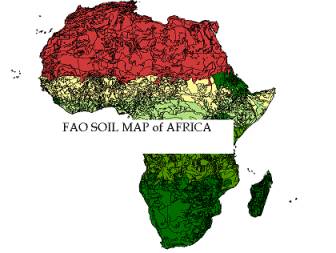
The FEWS Stream Flow (SF) Model is a spatially-lumped continuous, soil moisture accounting model. Inputs to the model includes NOAA (Climate Prediction Center) estimates of daily rainfall totals, USGS-developed global land cover, 1-kilometer DEM (HYDRO1K), and FAO soil layer at 1:1,000,000 scale (USGS Eros Data Center). The model consists of two parts: a GIS-based module used for model input and data preparation, and the rainfall-runoff simulation model.
Gulied A. Artan of the USGS provided the following files: basin.txt, evap.txt, fewsflood.avx, parameter2.txt, rain.txt, response.txt, route2.exe and schema.ini. The fewsflood.avx file was added to the EXT32 folder of ArcView. This is the GIS-based module used to extract physical parameters from grid datasets. The route2.exe file is the rainfall-runoff simulation portion of the model.

The runoff module divides the soil into an active soil layer and a groundwater zone. Runoff is generated by surface water due to precipitation excess, interflow and baseflow. Surface runoff, rapid sub-surface runoff flow and groundwater routing are modeled as linear reservoirs. For routing in main river reaches a non-linear formulation of the Muskingum-Cunge channel routing is used (USGS FEWS Model).
The first stage of this project was to closely examine the components of the model to determine how each worked. Once fewsflood.avx was added to the Arcview EXT32 folder, it could be added as an extension to the View window. The options included for the GIS-portion of the model include the following:
Option 1 generates all the necessary grids from the original DEM. Option 2 creates the basin.txt file. Option 3 creates the response.txt file. Options 4 and 5 create the rain.txt and evap.txt files. Option 6, Perform Flow Routing, runs the route.exe file. Option 7 computes rain and evaporation statistics by utilizing the rain.txt and evap.txt files. The last few modules of the model had unclear input file information, and gave errors. Option 10 however did create a Zone of Influence Grid and Flooded Area Grid, although these do not appear to be correct. The last option, Display Flow Hydrographs, did not work at all.
The files basin.txt, evap.txt, parameter2.txt, rain.txt and response.txt contain data for the Limpopo basin in Mozambique. The data are organized by level 5 Pfafstetter codes. The following table shows the fields included in each text file.
To run route2.exe (the runoff module) the file must be placed in a folder with basin.txt, evap.txt, parameter2.txt, rain.txt, response.txt and schema.ini. Running route2.exe creates the following files:
All these files are for daily time steps from 1999001 (January 1st, 1999) to 2001061 (791 days).
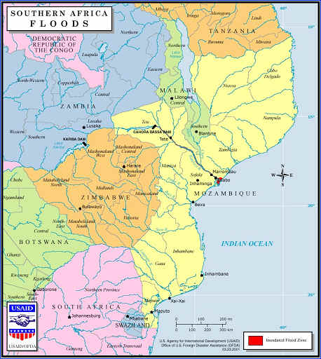
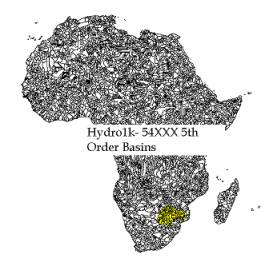
The HYRRO1K data provide basin boundaries and stream networks that form the spatial framework of the model. These data are in Lambert Azimuthal Equal Area projection and can be downloaded from http://edcdaac.usgs.gov/gtopo30/hydro. Opening these files was done with the help of a document written by Jordan Furnans. These data were downloaded for all of Africa in zipped format. Once unzipped, the files contained were af_dem.bil, af_dem.blw, af_dem.hdr and af_dem.stx. The imagegrid function in ArcInfo Workstation was used to convert the the .bil file to a grid. This function uses the other .hdr, .stx and .blw files to create the grids. Once these were in grid format, the ArcInfo Workstation Grid was used to correct for negative elevations and to assign NODATA values to ocean cells. The picture below shows the Hydro1K data for Africa. Mozambique is shown in yellow.
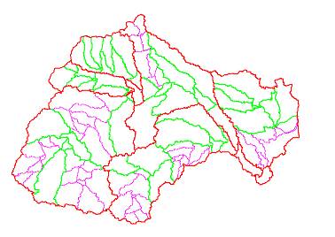
In order to match the data provided by Gulied A. Artan, the different basins were queried that had Pfafstetter codes greater than or equal to 54000 and less than or equal to 54999 using ArcView. The picture below shows the study area in relation to Mozambique.

The following pictures shows the level 3 Pfafstetter basins (in red), the level 4 Pfafstetter basins (in green) and the level 5 Pfafstetter basins (in pink).
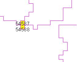
One problem encountered with the Hydro1K were one-cell basins, as shown below. The FEWS SF Model will not accept any one-cell basins as an input to the model.
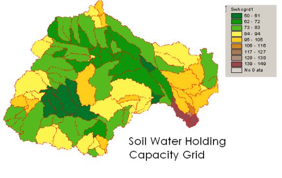
These data were originally in geographic coordinates. This map provides a characterization of the hydraulic properties of the earth's surface that are required to calculate the water balance within a basin. Needed to interpret these data are the Derived Soils Properties files. These files consists of interpretation programs written in QuickBASIC version 4.5. Using these programs parameters such as pH, organic carbon content, C/N ratio, soil depth, soil moisture storage can be interpreted.
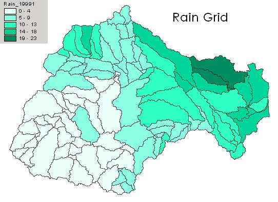
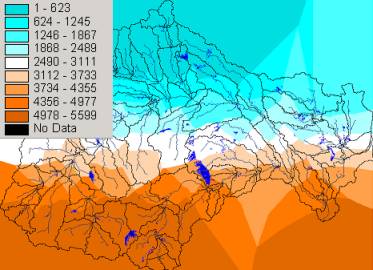
These data provide the estimates of gross precipitation into each basin. Data are provided daily for 10-day rainfall estimates.
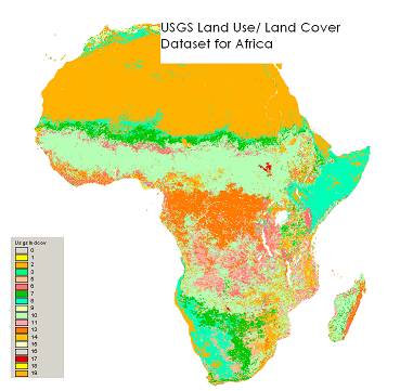
USGS Land Use/Land Cover System Legend (Modified Level 2). The
scrolling text box below contains the numbers displayed in the above figure,
with the corresponding land use/land cover type.
In order to apply the GIS portion of the FEWS SF model, input data was needed. As mentioned earlier, no information was available on this model, the input data required, nor the format that the input data should be in. Although the FAO Soils Map and USGS Land Use/Land Cover Datasets for Africa were prepared for use in the model, data already supplied in text format by Gulied A. Artan were used to assure consistent units.
Each grid was made by using the values from the basin.txt file. This file contains attribute values for each Pfafstetter basin. These values (eg CN for curve number) were saved as a .dbf file in Excel. In ArcView the fields were joined to the attribute table of the Pfafstetter basins, a new field created named after the attribute (eg CN for curve number), and the attributes then copied to this field. The resulting shapefile was then converted to a grid.
|
Curve Number Grid |
|
The Soil Water Holding Capacity Grid |
|
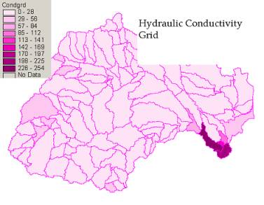
Hydraulic Conductivity Grid |
|
Soil Depth Grid |
|
Max Impervious Cover Grid |
This grid was zero for all basins.
|
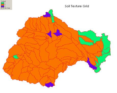
Texture Grid |
|
Velocity Coefficient Grid |
All values were set to equal 1.
|
Rainfall Grid for January 1st, 1999 (DAY 1) |
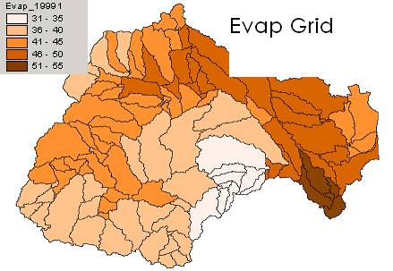
Evaporation Grid for January 1st, 1999 (DAY 1) |
The following diagram shows the change in evaporation and precipitation of the course 791 days. Only day 1 (January 1st, 1999) was converted to a grid.
Complete Terrain Analysis |
The first step, Complete Terrain Analysis, requires at a minimum the Hyro1K DEM. The option allows the user to also supply the Flow Direction Grid, Flow Accumulation Grid, Downstream Flow Length, Stream Grid, Stream Link Grid, Outlet Grid, Subbasin Grid, Hill Length Grid, Hill Slope Grid, and/or Downstream Grid. The output grids are those not provided in the input. In this case the following grids (and one shapefile) were computed: Downstream Grid, Hill Slope Grid, Hill Length Grid, Basins (Subbasin Grid), basply.shp (Vectorized Basins), Outlets (Outlets Grid), StrLinks (Stream Link Grid), Streams (Stream Grid), FlowLen (Downstream Flow Length Grid), FlowAcc (Flow Accumulation Grid), and FlowDir (Flow Direction Grid). The model renames the DEM to Elevations. The first time this step was done using a 1000 cell threshold. As one-cell subbasins were are problem in subsequent steps, a threshold of 3000 cells was used. The sinks were not filled in the DEM because the Hydro1K data has already been processed.
Generate Basin Characteristics File |
The second command, Generate Basin Characteristics File, generates the basins.txt and order.txt files. The inputs area the Basins Grid, the processed DEM (Elevations), the Flow Accumulation Grid, the Hill Length Grid, the Hill Slope Grid, the Runoff Curve Number grid, the Water Holding Capacity Grid, the Soil Depth Grid, the Hydraulic Conductivity Grid, the Downstream Flow Length Grid, the Stream Link Grid, the Downstream Grid and the Max Impervious Cover Grid.
Generate Basin Response File |
The third function, Generate Basin Response File, creates the response.txt file. This requires an input of the Velocity Coefficient Grid, and the grids created in Step 1: Basins Grid, Flow Direction Grid, Slope Grid and Stream Outlet Grid.
Interpolate Station Data to Grid and Generate Rain/Evap Data Files |
The Interpolate Station Data to Grid function was not used. Instead a grid was made using the data already provided. The Generate Rain/Evap Data Files creates the rain.txt and evap.txt files. The required inputs are the Basin Grid, and the individual Rain and Evaporation Grids. These must be named as rain_19991 and evap_19991 for the first day in 1999. Each day must contain a grid with this name format for the data to be added to the corresponding text file. The user can choose to extract rain and evaporation, or just rain or evaporation.
Perform Flow Routing |
For Perform Flow Routing the following inputs are needed: the length of model run in days, the number of subbasins, Manning's n, the fraction of active topsoil, the simulation start year, the simulation start day and the initialization mode (0 or 1).
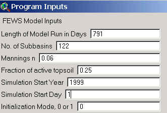
This is the point when it was discovered that route2.exe must be placed in ArcView's bin/ext/work directory. All the data files created in previous step were also placed in (rain.txt, evap.txt, response.txt, along with parameter.txt, schema.ini and route.exe) in the bin32 folder of ArcView. The FEWS SF Model, however, didn't seem to accept the initialization mode number. The parameter.txt file has written that this value is "0" for "no initialization data" and "1" for "read initial value of model state variables from a file." Neither value, 1 nor zero, were accepted by the model. An error message kept appearing ("a value of 0 or 1 must be entered") although these numbers had been entered.
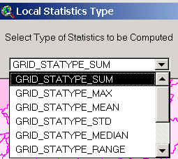
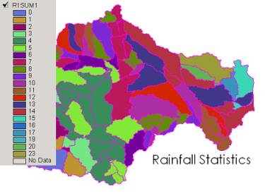
Compute Rain/Evap Statistics |
This is done by entering the following information:
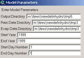
For each day there must be a corresponding grid. In this case statistics for only January 1st, 1999 were calculated. Next the parameters to extract are selected (rain, evaporation or both). For this step only rainfall was selected.
Compute Flow Statistics and Display Flow Percentile Map |
The next command, Compute Flow Statistics, first requires an input file. The input file required is not specified. Next the user is asked if he/she wants to convert highflow/lowflow thresholds. No was entered. The next input needed is the Basins Grid. This part of the model caused problems, even when different text files were used as inputs. The Display Flow Percentile Map could not be shown for the same reason as above: input files were not clearly specified.
Display Flooded Area Map |
For the Display Flooded Area Map first the Processed DEM is selected, then the Stream Links Grid, and the Flow Accumulation Grid. The flow depth data file is then asked for. The riverstage.txt was added as input. Next the user is asked what day the flood area is to be calculated for. The day 1.999e+6 is selected (the first option on the list). As a result two grids are created: a Zone of Influence Grid and a Flooded Area Grid. These grids were created without any error messages, but are most likely inaccurate.
Display Flow Hydrographs |
This last option did not work.
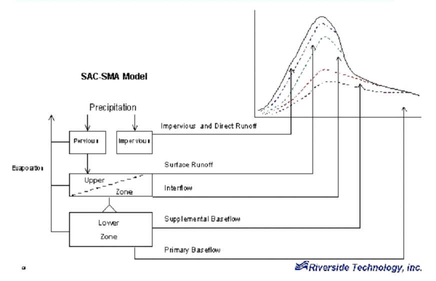
The rainfall-runoff prediction model contains three parts. The first is a soil water accounting module that produces surface and sub-surface runoff for each sub-basin . The second is a an upland headwater basins routing module which models surface runoff, rapid sub-surface flow and groundwater as three linear reservoirs. The third is a major river routing module. (USGS FEWS SF Model)
Similar to the Sacramento Soil Moisture Accounting Model (SAC-SMA), the soil is composed of two main zones: an active soil layer and a groundwater zone. The upper (active) zone represents short-term capacity and the lower zone represents the bulk of the soil moisture and longer groundwater storage. Each layer includes tension water elements (water bound by adhesion and cohesion), and free water elements (those that are free to move under gravitational forces and may be depleted only by evapotranspiration, percolation from the upper zone to the lower zone, horizontal flow and groundwater flow). In the upper layer evaporation, transpiration, and percolation take place. In the lower layer only transpiration and percolation take place. (USGS FEWS SF Model)

Source: http://meteora.ucsd.edu/~knowles/html/land/mod_descr.html
The soil moisture budget can be calculated as
The streamflow divergence R(t) consists of a surface runoff component S(t) and a subsurface component B(t).
![]()
Where W(t) is the soil water content at time t, P(t) is the mean precipitation over area A, E(t) is the mean evapotranspiration over area A, R(t) is the net streamflow divergence from area A, and G(t) is the net groundwater loss (through deep percolation) from area A. E(t) depends mainly on the net radiative heating on the surface and can be estimated by the Penman-Monteith equation. The runoff producing mechanisms considered in the model are surface runoff due to precipitation excess, interflow and baseflow. (USGS FEWS SF Model).
The following table shows the values included in parameter.txt. From these values the soil moisture budget parameters such as initial wetness, the pan evaporation coefficient, recharge and the fraction of the top soil can be altered for different areas.
|
Value |
Parameter in Parameter.txt |
|
16 |
MAXPAR (number of model static parameters) |
|
791
|
MAXTIME (number of days of model run) |
|
1999 |
begyear (simulation beginning year) |
|
1 |
begday (simulation beginning day of the year) |
|
112 |
MAXSUBASIN (number of sub-basins) |
|
2000
|
MAXLINE (maximum length of an output printed line) |
|
1000
|
MAXTOPOL (data level of the Pfafstetter topological
system for HYDRO1K) |
|
0.06
|
Manning (Manning coefficient) |
|
0.25
|
soil2top (fraction of the top soil layer of the
hydrologically active soil layer) |
|
0.5
|
recharge (model parameter to calculate groundwater
loss to regional flow) |
|
24.0
|
hour2day (number of hours in a day) |
|
0.95
|
Kc (pan evaporation coefficient) |
|
0 |
model initialization model |
|
0.80
|
InitialWetness |
The following diagram, provided by Riverside Technology, inc. shows the different runoff producing mechanisms and their individual contributions to the total runoff.
 .
.
The following two graphs (the same graph at different scales) show the different proportions attributed to each runoff mechanism over the period of 791 days used in the model.
As mentioned earlier, three linear reservoirs are used to model surface runoff, rapid subsurface flow and groundwater routing. The Muskingum-Cunge method, a simple diffusion type model, is used for river routing. This can used where backwater effects or reverse flows can be neglected (Maidment 1993).
Below is an example of how the FEWS Stream Flow (SF) Model can be applied to the ArcGIS Hydro Data Model. Level 5 Pfafstetter basins become Catchment, Level 3 Pfafstetter basins become Watershed, and Level 1 Pfafstetter basins become Basin in the Drainage Areas portion of the model. Under Hydro Features, the FAO Soils Map data and USGS Land Use/Land Cover data become FAOSoilDerivedFeatures and USGSLULCDerivedFeatures respectively. Under Hydro Network the raster derived Level 5 "streams" become HydroEdge.


In the FEWS SF Model, no channel geometry is needed. For this reason Channels is not included.
This model will be a very simple and straight-forward model to use once a user's guide is written. The user interface needs some development at this point in time. The model presents confusion as to what data to enter when, and the format the data needs to be in. Errors also occurred that could have been a result of bugs in the model (ie, not allowing the user to enter the initialization mode).
All in all, this model has a wide range of applicability in basins of large size. Apart for also being very flexible in terms of the location it is to be used in, all data can be obtained over the internet.
Georgakakos, Konstantine P, Jin Huang and Huun van den Dool. Analysis of Model-Calculated Soil Moisture over the United States (1931-93) and appliation to Long-Range Temperature Forecasts. Journal of Climate, Vol 9, No. 6, June 1996.
USGS global land cover characteristics database (http://edcdaac.usgs.gov/glcc/glcc.html);
FAO digital soil map of the world (http://www.fao.org/ag/agl/agll/prtsoil.htm);
FEWS Flood Risk Monitoring Model (http://edcsnw3.cr.usgs.gov/ip/gflood/ and http://edcsnw3.cr.usgs.gov/ip/fewsfloodrisk/index.html)- USGS EROS Data Center
Maidment, David R. Handbook of Hydrology, 1993 McGraw-Hill
Riverside Technology
Gulied A. Artan
Jordan Furnans