 (3.1a)
An atmospheric water balance is an accounting of the inflow and outflow of water vapor flowing over a region, coupled to the rate at which water is being added to or removed from the atmosphere by means of evaporation and precipitation. The percentage of the moisture flowing over a region which is involved in the region's hydrologic cycle can thus be assessed, and it may even be possible to estimate the rate of regional evaporation using measured atmospheric moisture flow and precipitation data.
Two sources of atmospheric data were used in this study. One data set was provided by Allen Bradley at the University of Iowa Institute for Hydraulic Research and the other by the National Meteorological Center (NMC). The data provided by Bradley originate from rawinsonde soundings. These rawinsondes are launched twice daily (0 and 12 Coordinated Universal Time (UTC)) to measure temperature, humidity, and wind profiles at several levels in the atmosphere. Using these data, Bradley estimated the specific humidity at each measurement level and used the following equations to estimate the vertically integrated vapor flux:


In these equations, Qu is the zonal (east-west) component of vapor flux in [kg m-1 s-1], Qv is the meridional (north-south) component of vapor flux in [kg m-1 s-1], q is the specific humidity [gm gm-1], u is the zonal component of wind velocity [m s-1], v is the meridional component of wind velocity [m s-1], p is the pressure [Pa], and g is the gravitational constant ( 9.81 m s-2 ). The negative sign arises due to the fact that the hydrostatic assumption was used to convert from elevation to pressure. The limits of integration are the surface pressure (ps) and the pressure at the "top" of the atmosphere (pt). Strictly speaking, the top of the atmosphere does not exist since there is no physical boundary constraining the atmosphere below a certain level; however, the transport of water vapor across the 300 mb (30.3 kPa) level is considered negligible so 300 mb was defined as the top of the atmosphere in these computations.
Bradley provided mean monthly integrated vapor flux values for October 1972 to December 1994. The mean monthly values for 0 and 12 Coordinated Universal Time were provided separately. These two values were averaged to estimate mean monthly flux. The data files from Bradley were provided in two formats: integrated flux estimates interpolated to a 2 grid using a standard meteorological method for interpolation called the Barnes objective analysis, and flux estimates interpolated to points on the Texas border from the 2 grid using bilinear interpolation. These two data formats facilitate computation of the atmospheric water balance using either a divergence approach or a flux integration approach as described below. Computations were made using both approaches as a check, and the two methods yielded consistent results.
Another data set, containing monthly atmospheric moisture divergence estimates on a 2.5 grid, was obtained from the National Meteorological Center (NMC) for the 26 month period from June 1991 to July 1993. At NMC, a general circulation model (GCM) is run two to four times per day to predict atmospheric conditions a few hours in advance. After these few hours have passed, observational data including rawinsonde data, satellite temperature and moisture data, and surface observations, are used to adjust the predictions and the next simulation is run. A general circulation model fills gaps in regions with sparse observations and creates atmospheric data sets on regular grids. The NMC monthly divergence estimates used in this study are outputs from the general circulation model. These values are the results of a simulation only and were not modified after the fact to fit actual measurements (Patoux, 1994). No computations were required to determine the divergence on the NMC grid because these values were provided; therefore, the calculations described below refer only to the Bradley data.
The mass conservation equation for water vapor in the atmosphere can be written as

where W is the amount of water vapor stored in the atmospheric
column, 


In Equation 3.3, H is the depth of liquid water storage in the basin, Rin and Rout are the inflow and outflow of surface or subsurface runoff, E is evaporation, and P is precipitation. Combining Equations 3.2 and 3.3 yields the expression:

In mean annual water balance computations, the change
in atmospheric storage (


It is seen in Equation 3.5 that if the divergence (
3.2.2 A Control Volume over Texas
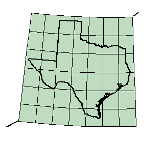
To define an atmospheric column for vapor flux calculations, the boundary of Texas was generalized by dividing it into straight segments, each with a length of approximately 100 km, and this boundary was extended vertically to the top (300 mb level) of the atmosphere. In visualizing this control volume, it is important to keep in mind that the height of the atmosphere (8-10 km) is thin compared to the horizontal extent of Texas. Figure 3.1 shows that only 42 2 cells are required to cover the state of Texas and surrounding areas, while Figure 3.2 shows the thickness of the atmosphere relative to the horizontal extent of a 2 grid cell.

3.2.3 Direct Computation and Flux Integration Approaches to Estimate Divergence
Two methods for computing divergence ( 


Re is the radius of the model earth taken as 6371.2 km, Ql and Qf are the zonal and meridional components of vapor flux (previously denoted as Qu and Qv respectively), l is longitude in radians, and f is latitude in radians. The spherical form of the divergence equation can be derived following the methodology given by Kreyszig, 1993, Section 8.12. The following centered difference approximation was used to calculate divergence directly from the 2 gridded data.

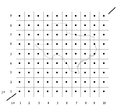
The 10 x 9 computational mesh used for the Bradley data is shown in Figure 3.3. For points on this mesh in columns 1 and 10 (i = 1 and 10) and rows 1 and 9 (j = 1 and 9), Equation 3.7 was modified to use a forward or backward difference approximation as appropriate, because data values outside of this mesh were not provided. The use of a forward or backward difference approximation did not affect any of the cells intersecting the boundary of Texas.
The units of the divergence computed with Equation 3.7 are [kg m-2 s-1]. To estimate the net divergence in the atmosphere above Texas, cells centered on the mesh points depicted in Figure 3.3 were intersected with the Texas boundary as shown in Figure 3.4. The boundary of Texas shown in Figure 3.4 is the same generalized boundary use in the flux integration calculations described in the next section. Intersection is a GIS term that describes an overlaying of two spatial data sets. In this case, the border of Texas was intersected with the 2 cell layout of atmospheric data to determine the area of each cell lying within the State. By summing up the divergence estimates and using these included areas as weights, an estimate of the divergence for the State as a whole was made. This intersection was made in a projected plane; the projection used was an Albers equal-area projection.

3.2.3.2 Flux integration approach
Thanks to the divergence theorem of Gauss (Kreyszig, 1993, p. 545, 551), an alternative method for calculating divergence is available that involves calculating the moisture flux across line segments that make up the Texas border. This approach is interesting because the flux across any arbitrary boundary line can be estimated. Because a three dimensional problem was reduced to a two dimensional problem through vertical integration of the vapor flux, the divergence theorem in two dimensions can be applied:

Rather than using a vector dot-product as in Equation 3.8, the right hand side of this equation can be evaluated by applying a vector cross-product to each border segment and summing the result for each to determine the net flux into the Texas atmosphere. This concept is illustrated in Figure 3.5.

The vector 

In this problem, the boundary segments that make up the
border of Texas are defined so that they all point in a clockwise direction,
the interior of the region is to the right of each boundary vector and
the exterior to the left. The result of the vector cross product is a vector
oriented in the vertical direction. If this vector is positive, this indicates
mass leaving the region and if this vector is negative, this indicates
mass entering the region. For net flux calculations, only the magnitude
of the resulting vector 


In these calculations, the directions of the vector flux components are defined in geographic space and the geometric relationship between the flux vectors and border segments is also determined in geographic space; however, the lengths of the border components |lx| and |ly| correspond to the length of these segments as measured along the surface of the earth. To estimate |lx| and |ly| given the latitude and longitude of segment endpoints, the length of a radian of longitude and a radian of latitude on the earth's surface (with the earth represented as an ellipsoid) were multiplied by the difference between the longitude and latitude of the two segment endpoints as follows:


The equations for the length of a radian along a meridian
of longitude and the length along a parallel of latitude were taken from
Snyder, 1987, p. 25. The parameters for the Clarke 1866 ellipsoid were
used to evaluate Equation 3.10 because this was the ellipsoid used to define
the Texas border. In Equation 3.10, a is the radius of curvature
for the ellipse in the plane of the Equator (a=6378206.4 m), e
is the eccentricity (e=0.000045815), 

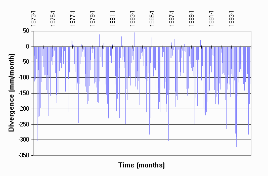
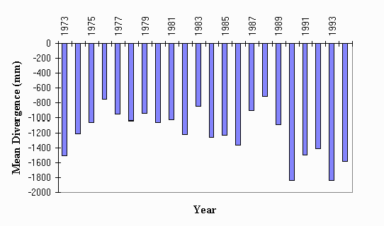
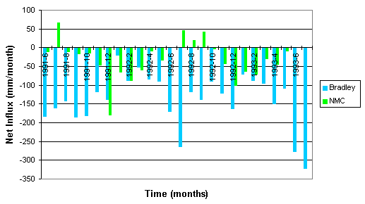
Figure 3.6 shows the results of the monthly divergence calculations for 1973 to 1994 using the Bradley data. These are the results from a direct divergence calculation on a spherical grid (Section 3.2.3.1). Although not shown here, the flux integration results (Section 3.2.3.2) are nearly identical (within 2% on average) as expected. Figure 3.7 presents the same data of Figure 3.6 averaged by year. Figure 3.8 provides a comparison of Bradley and NMC divergence for the 26 month period when the NMC data were available (June 1991 - July 1993). There are significant differences between these two estimates, both in variation of divergence throughout the year and the average divergence magnitudes. Assuming that the mean annual change in atmospheric storage is negligible, the 22 year average runoff (P-E) from the Bradley data is 1206 mm year-1 and the 2 year average runoff predicted from the NMC data is 379 mm year-1. Both of these estimates are much higher than observed surface runoff. A 30 year mean annual runoff of 78.4 mm year-1 was estimated from the surface water balance described in Section 5 below. Such large errors in predicting runoff using the atmospheric water balance are not uncharacteristic for this type of study. Although Oki et al. found good agreement between convergence and observed runoff for several basins in the analysis of 70 basins worldwide, they also reported a wide range of errors in which the vapor flux convergence may be up to 80 times the observed runoff or the vapor flux convergence may predict a net evaporation 28 times greater than observed runoff. Several sources of error in making atmospheric flux calculations are discussed in Section 3.3.2.
If it is assumed that the change in storage from month
to month in the atmosphere is negligible, an evaporation estimate can be
made as (E = 


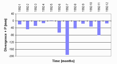
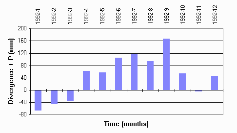
Unfortunately, very little data on atmospheric storage were available for this study. In unpublished follow-up work to the study by Patoux, 1994, Patoux estimated the moisture content of the atmosphere over Texas for the first 6 months of 1991. The moisture content increased from about 17.1 mm in January to 54.7 mm in June, with increases of 3.6 mm, 2.4 mm, 3.4 mm, 7.8 mm, and 20.4 mm in the intervening months. This trend simply shows that the atmosphere holds more moisture in the warm summer months. It doesn't appear that large discrepancies illustrated in Figures 3.9 and 3.10 can be explained by these relatively modest atmospheric moisture changes.
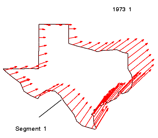
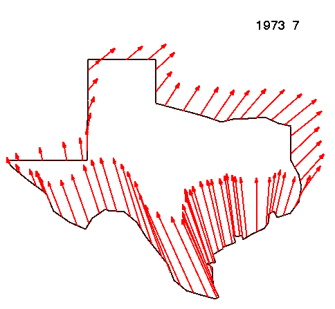
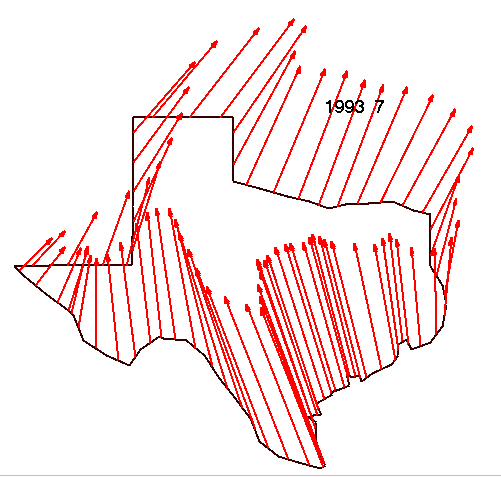
In addition to making net flux calculations, a simple program for displaying flux vectors in a geographic information system was developed for use in this study. Looking at the flux vectors gives a sense of where moisture enters and leaves the State, and also gives a feel for seasonal and annual trends in moisture flux magnitudes. Figures 3.11 and 3.12 show moisture flux vectors for January and July 1973. The moisture flow over Texas drastically increased during the Midwest flood of 1993 which is shown in Figure 3.13. Comparing Figures 3.12 and 3.13 shows the difference in summer moisture flux between 1973 and 1993.
The sparseness of observation points, both horizontally and vertically, leaves room for significant error in the atmospheric flux calculations. Even if estimates at all the 2 grid points are accurate, this leaves only about 42 observations, after vertical integration, to describe the flux over an area of 690,000 km2. In addition to problems with sparseness of measurements in the horizontal direction, Brubaker et al. note that the vertical resolution of atmospheric soundings, which typically include measurements at about 6 levels from 1000 to 300 mb (about 0 - 10 km), do not adequately resolve the atmospheric boundary layer (for which a typical depth is 1 km) where a large fraction of the atmospheric water vapor can be found.
Because of the large magnitudes of the numbers under consideration, a small error in the estimate of vapor flux across a single line segment may have a relatively large impact on the net influx computation. For example, the flux across segment 1 (86 km) in Figure 3.11 is 9.180 x 10⁶ kg s-1 which is equivalent to about 9810 m3 s-1 or 36 mm month-1 when dividing by the area of the region being considered this value is significant when compared with the netflux estimates given in Table 3.1 below. The fact that there are large volumes of water both entering and leaving the State means that calculating the net influx requires taking the difference between two large numbers of similar magnitude. As a result, a small percentage error in either the total influx or total outflux estimate can lead to a large percentage error in the result. Table 3.1 was constructed using data from 1977 to illustrate this point. The netflux is (outflux - influx) and the throughflux is (outflux + influx)/2.
Table 3-1: Comparison of Netflux and Througflux in 1977
| Month | Influx (mm) | Outflux (mm) | Netflux (mm) | Throughflux (mm) | |Throughflux/Netflux| |
| 1977-1 | 665.0 | 668.7 | 3.8 | 666.9 | 178 |
| 1977-2 | 416.2 | 419.7 | 3.4 | 418.0 | 122 |
| 1977-3 | 928.3 | 867.2 | -61.0 | 897.8 | 15 |
| 1977-4 | 624.2 | 540.2 | -84.0 | 582.2 | 7 |
| 1977-5 | 926.1 | 786.4 | -139.7 | 856.2 | 6 |
| 1977-6 | 738.4 | 618.9 | -119.4 | 678.6 | 5.7 |
| 1977-7 | 715.0 | 594.6 | -120.4 | 654.8 | 5.4 |
| 1977-8 | 819.5 | 577.7 | -241.9 | 698.6 | 2.9 |
| 1977-9 | 603.4 | 480.1 | -123.3 | 541.7 | 4.4 |
| 1977-10 | 603.0 | 545.6 | -57.5 | 574.3 | 10.0 |
| 1977-11 | 500.3 | 471.9 | -28.4 | 486.1 | 17.1 |
| 1977-12 | 732.3 | 737.4 | 5.0 | 734.8 | 145 |
Another source of error relevant to the analysis using Bradley data is that mean monthly flux values were used, meaning that transient eddy flux terms were not considered. When time averaging is done on the product of two time-varying quantities - like velocity and specific humidity in this case - eddy flux terms arise because of random variations in velocity and in specific humidity at time scales less than the averaging period used for the analysis. These eddy flux terms may have a significant influence on mass transport in certain situations. In their analysis of moisture flux into North and South America, Brubaker et al. decomposed the vertically integrated moisture flux into mean motion and transient eddy terms. They note that from a global perspective mean motion dominates Qu while mean and transient eddy terms are of comparable magnitude in Qv. From the results of their study, Brubaker et al. concluded that eddy flux terms contribute significantly to the north-south transport of water vapor, particularly along the Gulf of Mexico in the winter months. Thus, fluctuations on a few days time scale are important when considering the transport of water vapor, a conclusion also reached by Rasmusson, 1967.
Two methods for computing the divergence of atmospheric moisture using rawinsonde data have been described one using a finite difference approximation on a spherical grid and one by summing fluxes across boundary lines. The results of these computations were compared with output from a general circulation model. In general, computations based strictly on observed data yielded poor estimates of divergence, with the estimate of average annual divergence over Texas being 15 times greater than observed runoff. The divergence estimate from the general circulation model was about 5 times greater than observed runoff. Reasons for errors may include (1) the sparseness of observations, (2) errors associated with taking differences between large numbers, and (3) using monthly average flux values. With regard to the first reason for errors, improved observation networks and remote sensing may help to alleviate problems with data resolution in future studies. The United States National Meteorological Center is presently implementing a new mesoscale general circulation model over North America called the Eta model, using 40 km computational cells which will provide about 25 times greater horizontal resolution than the grid used in this study. The second problem may be difficult to overcome considering the large amounts of moisture that flow through the atmosphere relative to the amounts of precipitation, evaporation, and runoff. Statewide average estimates from this study indicate that the average annual throughflux (1973 - 1994) of atmospheric moisture is 7788 mm while the annual precipitation is 720 mm and average annual runoff is 78.4 mm (See Section 5), indicating that only 9% of the moisture passing over the State falls as precipitation and 11% of this precipitation becomes runoff. With regard to the third problem, data for making calculations on shorter than monthly time steps are available, but were not used due to time and logistical constraints in this study.
When calculations made in this study were compared with the output of a National Meteorological Center GCM, the GCM results seemed more reasonable, but not entirely satisfactory. The GCM considers transient eddy behavior that is not captured by mean monthly observations because a much smaller time step is used. Simulation models also offer the advantage that equations of motion can be used to fill in areas with sparse observations. As products from higher resolution GCM simulations become available, simple operations in GIS can be used to estimate net fluxes into arbitrarily defined regions as done in this study.
Some additional information would have been useful to help assess the relative importance of different sources of error in this study. The use of 12 hourly data could have shed more light on problems associated with using monthly average values. It also would have been interesting to know the locations where rawinsonde observations were actually made. In addition, more water content computations could have been made to yield better evaporation estimates.