![]()
 |
(1)
|
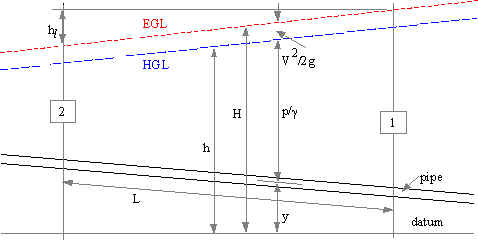
where a1, a2 = kinetic energy correction factors, which are dimensionless; V1, V2 = the cross sectional average fluid velocities at points 1 and 2, respectively; g = acceleration due to gravity; p1, p2 = pressures at points 1 and 2, respectively; z1, z2 = elevations above the datum at points 1 and 2, respectively; hf = head loss due to boundary shear; and hL = minor losses. This equation applies only for control volumes which are single streamtubes, i.e., control volumes with only one inflow and one outflow and with the inflow and outflow rates equal to each other.
Total head is defined as the rate at which kinetic and potential energy
are transported by the flow plus the rate at which the fluid does work
against the internal pressure, all divided by the rate at which the weight
of the fluid is being transported by the flow. That is,
 |
(2)
|
There is a similar relationship for any head (h), i.e.,
| h = P/gQ or P = gQh |
(3)
|
where h can be the frictional head loss, the pressure head, the head from a pump, etc., and P is the rate of doing work (e.g., against shear stresses or pressure) or the power (e.g., from a pump) or the rate of transport of energy (e.g., the rate at which kinetic energy is transported by the fluid when the head is the velocity head). All of the things that P can represent have dimensions of LF/T. Since h is defined only for single streamtubes and since h is obtained by dividing P by gQ, head is like an intensity in that it is associated with each unit of fluid. As a result, head is not divided between different flow paths when a flow splits nor is it additive when two or more flows come together.
 |
(4)
|
where f = Darcy-Weisbach friction factor, L = length of pipe, D = pipe
diameter, and V = cross sectional average flow velocity. This equation
is valid for pipes of any diameter and for both laminar and turbulent flows.
For laminar flow,
 |
(5)
|
where Re is the Reynold's number, which is defined for pipe flow as
|
(6)
|
Substituting flam and Reynold's number into the Darcy-Weisbach
equation yields
 |
(7)
|
For turbulent flow, the friction factor can be obtained from a Moody
diagram or from the Colebrook-White equation, which is
 |
(8)
|
where ks is the equivalent sand roughness and ks/D is the relative roughness. The values of f in the Moody diagram and in the Colebrook-White equation are empirical, i.e., they came from experiments.
 |
(9)
|
where K is an empirical minor loss coefficient. Some examples
of minor losses are the losses due to a pipe entrance or exit; an expansion
or contraction, either sudden or gradual; bends, elbows, tees, and other
types of fittings; and valves, either totally open or partially closed.
For many situations with two pipe sizes (e.g., expansions and contractions),
both the velocity in the smaller pipe is used in the text book for defining
the minor loss coefficient. Essentially all minor loss coefficients
are empirical. An exception to both the form of the minor loss equation
and to the necessity of obtaining minor loss information from experiments
is an abrupt expansion for which the momentum and energy equations can
be used to get the loss as
 |
(10)
|
where Va is the velocity in the smaller pipe (i.e., the larger
velocity) and Vb is the smaller velocity in the larger pipe.
A special case of an abrupt expansion is the exit from a pipe into a reservoir.
For this type of "expansion", Vb = 0 in the reservoir
so
 |
(11)
|
where V is the velocity in the pipe and K = 1.
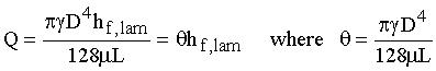 |
(12)
|
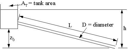
For a tank and tube as shown in Fig. 1, hf,lam = h if the
entrance loss and the velocity head at the downstream end of the tube are
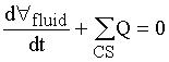
negligibly small. Taking the tank as a control volume, the continuity
equation gives
 |
(13)
|
Since the depth of liquid in the tank is h minus a constant (zb)
and since there is only one outflow,
 |
(14)
|
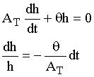
Substituting Eq. 12 for Q and separating variable, the result can be
written as
 |
(15)
|
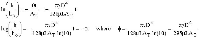
Integration with h = ho at t = 0 gives
 |
(16)
|
Measuring h as a function of time as a liquid drains from the tank and plotting h/ho on a semilogarithmic graph will produce a straight line when there is laminar flow in the tube. The slope of that line will be f. Determination of f will then allow m to be evaluated.
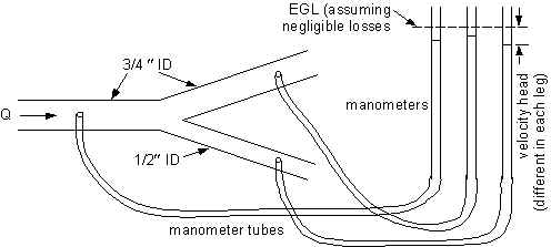
Fig. 2 - Schematic diagram of branching pipes to illustrate that head
is not divided between flow paths
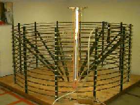
a) Photograph |
b) Schematic diagram |
Fig. 3 - Spiral pipe for measuring head loss due to boundary shear
 |
L1-2 = 550.5 cm
L2-3 = 22.2 cm L4-5 = 41.6 cm L5-6 = 1116.3 cm L6-7 = 20.6 cm L8-9 = 36.7 cm L9-10 = 551.5 cm |
![]()
 |
(17)
|
where Dh = change in piezometric head, R = manometer reading, gm = specific weight of manometer fluid, and g = specific weight of flowing fluid. Head losses are defined in terms of total head (H), not piezometric head (h), but the velocity head is constant for a constant diameter pipe, so Dh = DH. The change in total head between the two piezometer taps is the head loss.
|
(18)
|
using the measured head loss (hf = Dh), using the known values of L and D, and calculating V from Q and D.
|
(19)
|
|
(20)
|